How does an operating system determine how much processing time a single process receives? There are a number of fundamental “scheduling policies” that an architect of an operating system may consider implementing:
- first-come-first-served
- round robin
- shortest process next
- shortest remaining time
- highest response ratio next
For the sake of simplicity, we are going to focus on short-term scheduling on a multiprogramming system.
Terminology
What is a multiprogramming system?
A multiprogramming system is a basic form of parallel processing in which multiple programs are run at the same time on a uniprocessor. As a result of having only a single processor, concurrent execution of multiple programs is impossible. Rather, the operating system must alternate between the programs, e.g. giving some processing time to one process, then switching to a different process.
What is short-term scheduling?
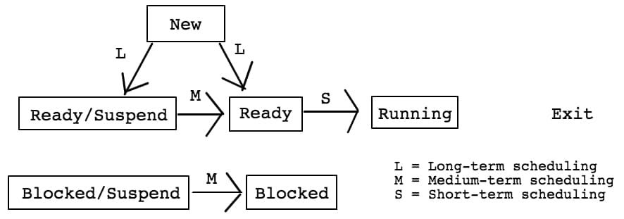
In order to understand short-term scheduling, it is helpful to step back and take a look at the bigger picture. Scheduling on most systems can be broken down into three separate tasks:
- Long-term Scheduling – The decision to add a new process to the group of processes to be executed. The greater the number of processes in the system, the smaller amount of time an individual process can be executed; as a consequence, competition for the processor increases.
- Medium-term Scheduling – The decision to add a process to the group of processes that are partially or fully in main memory. Part of the swapping function which exchanges the contents of an area of main memory with the contents of an area of secondary memory.
- Short-term Scheduling – The decision of which available process will be executed next by the processor. Invoked when the current process is at risk for being blocked or preempted which can be caused by clock interrupts, I/O interrupts, OS calls, or signals.
You can think of scheduling as managing queues of processes to minimize queueing delay and to optimize performance.
If the above was a bunch of text garbage, ignore it for now. You can still understand the scheduling policies covered without it. Just know two things:
- There are more types of scheduling than only short-term.
- Short-term scheduling is referring to how an operating system decides which process executes next on the processor.
Understanding the Selection Function
Each policy has a selection function, which is used to determine which ready process is selected next for execution. We will analyze each policy only by its execution characteristics, but in reality, there are additional factors to consider like priority and resource requirements. The following are execution characteristics we will consider:
- w = time spent in system so far waiting
- e = time spent in execution so far
- s = total service(execution) time required by the process
Exactly when the selection function is run depends on whether or not the scheduling policy is preemptive or nonpreemptive. For a nonpreemptive policy, once a process is running, it continues to execute until it terminates or it blocks itself; it is not interrupted. In preemptive policies, a running process can be switched out for a different process before it finishes based on a particular scheduling policy’s unique preemptive condition. A preemptive condition can be things like a clock interval or the arrival of a new process to the ready pool.
An Introduction to Scheduling Policies
First-come-first-served (FCFS)
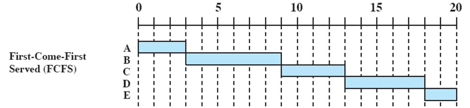
First-come-first-served is nonpreemptive and characterized by the selection function max[w]. FCFS is just another way of saying first-in-first-out(FIFO). This means that the process that has spent the most amount of time waiting will be the one to execute.
| Process | Arrival Time | Execution Time |
|---|---|---|
| A | 0 | 3 |
| B | 2 | 6 |
| C | 4 | 4 |
| D | 6 | 5 |
| E | 8 | 2 |
Looking at the execution pattern, process A starts at time slot zero, since FCFS is non-preemptive, process A will execute until it ceases to execute. Process B arrives at time slot 2, but it can’t preempt process A, so it must wait for process A to terminate, which terminates at time slot 3.
Once process A terminates, because it has been waiting longer than any other process, process B is selected for running (there are no other processes in the system). The pattern continues, and process B, will also execute until it terminates, or in an additional 6 time steps at time slot 9.
Processes C, D, and E, all arrive while process B is executing, but at the time process B terminates, C is waiting for 5 time steps (w=5), D for 3 time steps(w=3), and E, for 1 time step(w=1). So applying our selection function max[w], process C will be selected. The pattern continues, until all processes are serviced.
Round Robin (RR)
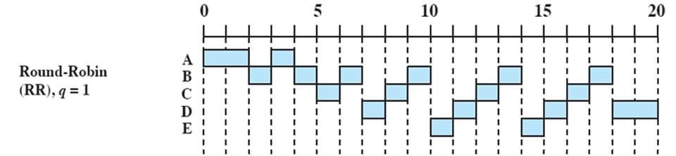
Where FCFS was nonpreemptive, round robin uses preemption based on a clock. This means that there is a maximum amount of time that a single process can execute before it is interrupted and another process is allowed to run. It is helpful to imagine a group of ready processes sitting in a circle. They “share” a single processor. Each process gets an equal amount of execution time before passing on the processor to the next ready process.
| Process | Arrival Time | Execution Time |
|---|---|---|
| A | 0 | 3 |
| B | 2 | 6 |
| C | 4 | 4 |
| D | 6 | 5 |
| E | 8 | 2 |
This “sharing” is illustrated by the execution pattern, which has a time slice of q = 1. Process A arrives at time slot zero. Even though the time slice is only 1, there are no other processes in the system so process A is allowed to execute for 2 time steps. However, once process B enters at time slice 2, process A must stop executing, and hand the processor over to process B which then executes for 1 time step before giving it back to process A for a single time step. A is now finished executing at time step 4.
Something confusing happens at time step 4 though, because process C arrives into the system and we now have two processes, B and C, in the system. Which executes next? The round robin policy does not actually specify what should happen. Since for our purposes it is essentially arbitrary, we are going to assume they execute in alphabetical order. So B will execute for 1 time step, followed by C for 1 time step. The pattern continues, until all processes are serviced.
Shortest Process Next (SPN)
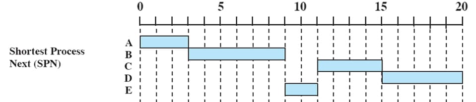
Shortest process next is a nonpreemptive policy characterized by the selection function min[s]. Simply put, the process that has the shortest overall expected execution time is selected next.
| Process | Arrival Time | Execution Time |
|---|---|---|
| A | 0 | 3 |
| B | 2 | 6 |
| C | 4 | 4 |
| D | 6 | 5 |
| E | 8 | 2 |
In the execution pattern example, at time slot 0, A is the only process in the system, so by default, it has the lowest min[s]. The policy, as stated earlier, is nonpreemptive, so A executes until completion. Process B enters at time slot 2 and waits for A to finish at time slot 3. Exactly similar to the scenario with process A earlier, B is the only ready process in the system, and so process B has the shortest expected execution time.
Once B terminates at time step 9, processes C(s=4), D(s=5), and E(s=2) are all now waiting. The operating system then applies the selection function min[s] again, which leads to process E executing. Later to be followed by process C, and lastly process D.
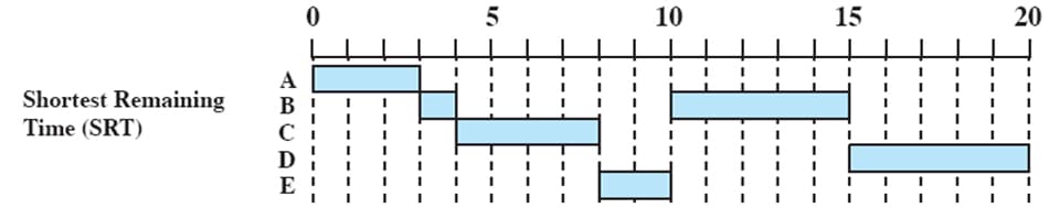
Shortest Remaining Time (SRT)
Shortest remaining time works similarly to shortest process next with one differentiating factor—it is preemptive. This gives a selection function of min[s-e]. Whenever a new process joins the ready processes, if it has a shorter remaining time than the currently running process, it will interrupt the current process and run instead.
| Process | Arrival Time | Execution Time |
|---|---|---|
| A | 0 | 3 |
| B | 2 | 6 |
| C | 4 | 4 |
| D | 6 | 5 |
| E | 8 | 2 |
In order to highlight this difference, let’s take a look at the SRT execution pattern. At time slot 0, process A is the only process so it starts. At time slot 2, process B comes in at which point the OS will run the selection function. For process A, s = 3 and e = 2, giving s-e = 1. For process B, s = 6 and e = 0, giving s-e = 6. 1 is less than 6, so process A continues to execute.
Process A terminates at time step 3, giving process B, the only ready process, a chance to execute for 1 time step before process C joins the ready processes at time step 4. The selection function runs again. For process B, s = 6 and e = 1, giving s-e = 5. For process C, s = 4 and e = 0, giving s-e = 4. 4 is less than 5, so process C starts to execute.
Process C continues to execute until time step 6, at which point the selection function is run again when process D enters the ready processes. Process B still evaluates to 5. For process C, s = 4 and e = 2, giving s-e = 2. For process D, s = 6 and e = 0, giving s-e = 6. C is still the lowest so it continues to execute.
Process C now continues until it both terminates at time step 8 and process E joins the ready processes. Process B still evaluates to 5 and D still evaluates to 6. For process E, s = 2 and e = 0, giving s-e = 2. E then executes for two time steps.
This pattern continues each time a new process is added to the ready process pool.
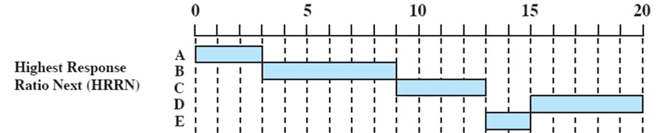
Highest Response Ratio Next (HRRN)
Highest response ratio next is a nonpreemptive policy with a selection function of max(w+s/s). For reasons I’m not going to explain in this blogpost, HRRN does a good job of accounting for the age of a process so that longer processes are eventually chosen over shorter processes.
| Process | Arrival Time | Execution Time |
|---|---|---|
| A | 0 | 3 |
| B | 2 | 6 |
| C | 4 | 4 |
| D | 6 | 5 |
| E | 8 | 2 |
Looking at the execution pattern, like our other examples process A enters at time slot 0 and executes. HRRN is nonpreemptive, so when B enters at time slot 2, A is uninterrupted and allowed to complete. At time slot 3, process B is the only process in the system and as a result, is selected by the selection function; it executes until completion.
When process B terminates at time slot 9, process C, D, and E are all in the system. For process C, w = 5 and s = 4, giving w+s/s = 5+4/4 = 2.5. For process D, w=3 and s = 4, giving w+s/s = 3+4/4 = 1.75. For process E, w = 1 and s = 2, giving w+s/s = 1+2/2 = 1.5. Process C has the highest value, and so it executes until completion.
This pattern continues every time a process terminates.
Conclusion & References
We ended up covering five different scheduling policies, but we didn’t compare, analyze, or go over the use-cases for each policy. If there is any interest, I would like to write another blogpost covering these topics. Regardless, understanding the workflow of each policy is a good start, and you may already be able to draw some of your own conclusions about their pros and cons.
I found this book invaluable while writing this post:
Stallings, William. Operating Systems Internals and Design Principles. New Jersey: Prentice Hall, 2012. Print.
Credit especially goes to the author for the examples I used for each scheduling policy. It saved me a lot of time not having to do each by hand. I highly recommend it for your personal bookshelf, the authors do a phenomenal job making textbook reading easy.