
I recently worked on a side project that exposed me to some of the more advanced aspects of Google Sheets. Eventually, I stumbled my way into Google Sheet queries, which solved my problem by allowing me to link data on multiple sheets. This post is meant to introduce you to some of the benefits of this feature, which might help you solve a problem down the road.
A query in Google Sheets allows you to view and manipulate a set of data. For example, if you had a list of places you wanted to see at a certain destination, you could write a query to return the top five places from highest to lowest ranked. Simply put, it lets you turn questions into data-backed results.
It also enables you to join data from multiple tabs, similar to H or VLOOKUP. I’ve put together some time tracking and employee data to show how this works. I created a new worksheet in Google Sheets and added several tabs. The Employee List tab has the fake employee data, the Punch Data tab has punches for each employee’s hours, and the Report tab is used for reporting.
To make working with the data easier, I suggest using Named Ranges to make aliases for the cell ranges which hold your data. I made two Named Ranges, one for the Employees and another for Punches. This eliminates the need to specify the tab name and the cell ranges each time you write a query.
To start the demo, let’s output all the daily time punches for each employee on the report tab. We can do this by entering the following into a cell:
=QUERY(Punches, "Select *")
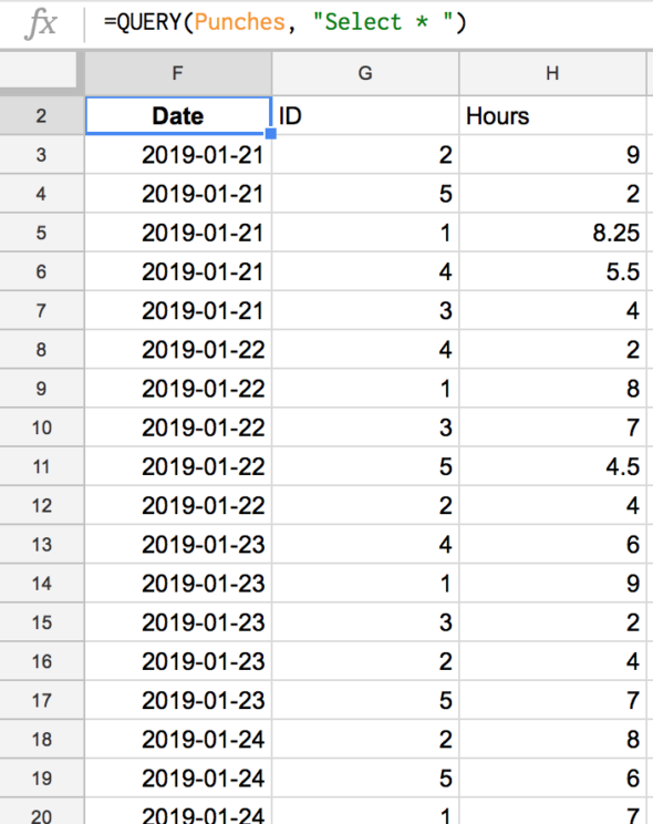
This should return all of the columns and rows from the data set. From here, you can manipulate the query to return only the desired columns of data. All you have to do is replace the * with your desired columns.
To return only the date and hours, we can just replace * with A, C. Notice now the ID column no longer appears.
We can then ask, “What is the total of all punches?” We can change the query again to "Select SUM(C)". This should total the punches in our data set and output the answer.
Let’s say we want to get a list of all punches for a particular employee. We could use the Where clause to filter the data being returned. So we’ll change the query to:
=QUERY(Punches, "Select * Where B=1”)
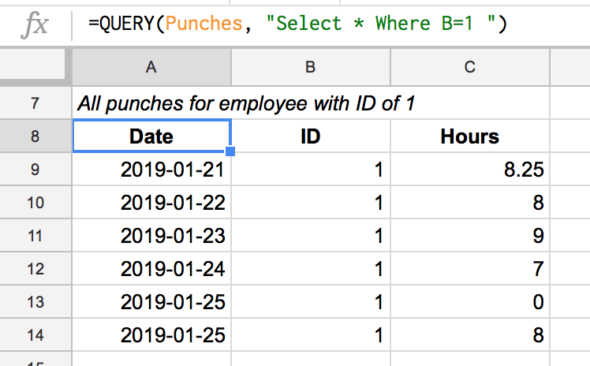
This will search our punch data and return all the columns of data where the ID is equal to 1, which accomplishes our task of limiting the data to a specific ID.
Next, we can look at some aggregate data. Try:
=QUERY(Punches, "Select B, SUM(C) Group by B ")
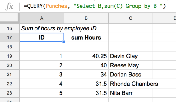
This lets us group the data together. The output shows us a list of IDs with the total of punches in the data.
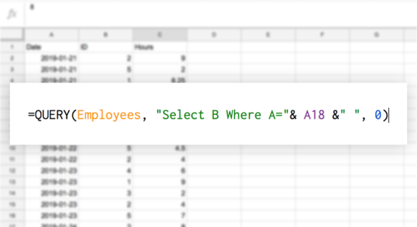
We can add another query to the result. In the next available column in the row of the first ID, we can ask Sheets to return the name of the employee whose ID is equal to 1.
=QUERY(Employees, "Select B Where A="& A18 &" ", 0)
This query looks through the Employee data to find the name of the employee from column B where the ID from column A is equal to the ID in the desired cell. In this case, it’s Cell A18.
Now that we can reference a cell, let’s make it easy for someone to select an employee name which returns a list of that person’s punches. In an empty cell, use Data > Data validation to allow users to only enter in a user’s name from the column of names in the Employee List tab. We can then query to get that user’s ID like this:
=QUERY(Employees, "Select A Where B like '"& B24 &"' ",0)
This query asks to search the Employee data to find the ID in column A that is like the name from column B that matches the user’s selected name from the reporting tab–in this case, from Cell B24. This will return the employee’s ID.
We can take that ID and use it in another query like the one we used above, but now we’ll reference the cell that returns the query to populate the data.
=QUERY(Punches, "Select A,C Where B="& B25 &" ")
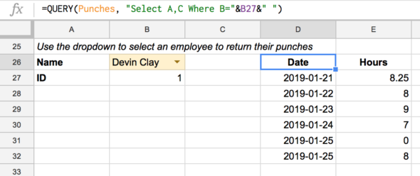
This query will then return the date and punches for the employee ID that is in Cell B25.
There are a slew of ways to alter your query, including some of the following:
- Selects all columns
- Where
- Operators
- Variables
- Order
- Limit data returned
- Group by
View a live version of the Google Spreadsheet here.
=QUERY({Sheet1!A2:D10;Sheet2!A2:D10;Sheet3!A2:D10}, “select col2 where col1=’ “&A2&” ‘ “)
im trying to get B2 from sheet2,sheet3
if A2 in sheet1 matches A2 in sheet 2/ sheet3
your example works for one sheet//
can you help me get this solution please
Hey Bryan, I would like to be a master of queries sql functions for google sheets but it very difficult to find this kind of material to study. Most that i found is about sql server and many of them dont work in google sheets. Could you point me more specific material?
Regards
Fabio