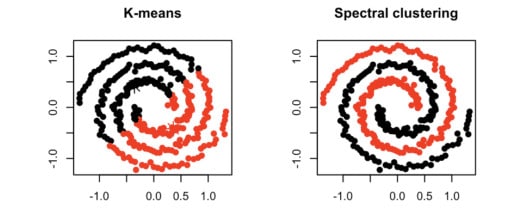
Clustering algorithms like K-means and Mean Shift are widely used in order to group data-points into compact clusters. However, when data isn’t “globular,” we need a method of grouping data by connectedness rather than compactness. In those cases, we can leverage topics in graph theory and linear algebra through a machine learning algorithm called spectral clustering.
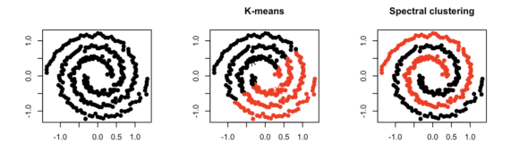
As part of spectral clustering, the original data is transformed into a weighted graph. From there, the algorithm will partition our graph into k-sections, where we optimize on minimizing the cost of removing edges to achieve the partition. Hence, we’re ultimately solving a min-cut graph problem.
Morphing Raw Data into a Similarity Graph
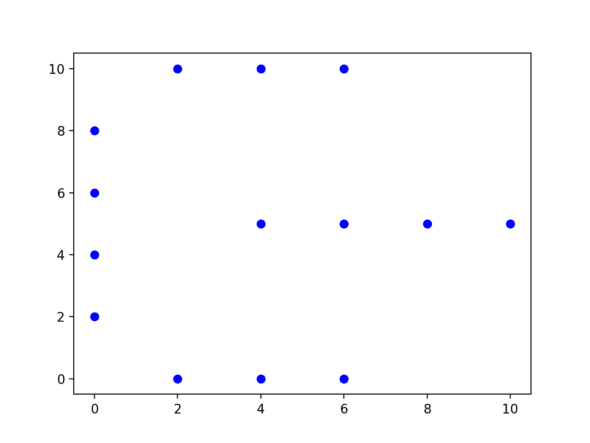
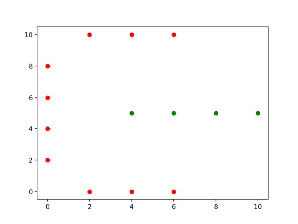
Let’s dive right into an example. Consider the following dataset:
class Point():
    def __init__(self, x, y, color="blue"):
        self.x = x
        self.y = y
        self.color = color

dataset = [Point(2, 0), Point(4,  0), Point(6, 0), Point(0, 2),
           Point(0, 4), Point(0, 6), Point(0, 8), Point(2, 10),
           Point(4, 10), Point(6, 10), Point(4, 5), Point(6, 5),
           Point(8, 5), Point(10, 5)]
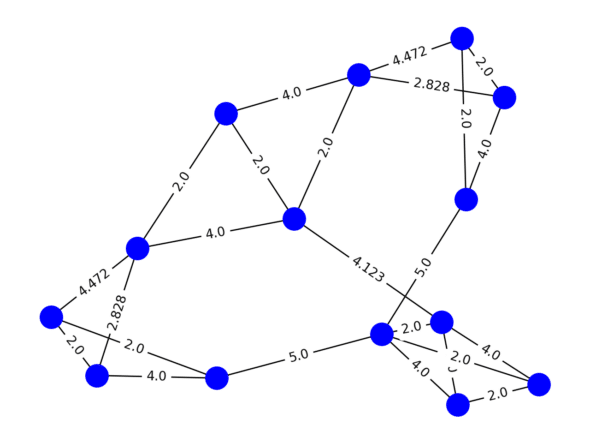
The first step of spectral clustering is to construct a graph based on some definition of similarity. To do so, define a function that takes input of any two nodes A and B and outputs a numeric representation of their similarity. That value will dictate the edge weight between nodes A and B in our graph. In our case, we’ll define similarity as the euclidean distance between the 3-Nearest Neighbors of each point, and 0 between non-neighbors. The sklearn library in Python helps us generate that graph in the form of a matrix in just a few lines.
from sklearn.neighbors import kneighbors_graph

points = [[point.x, point.y] for point in dataset]
graph = kneighbors_graph(points, n_neighbors=3, mode="distance").toarray()
Eigenvectors of the Laplacian
Now we’ve created a representation of our graph in the form of a weight matrix (W). Additionally, as is the case in other graph partitioning problems, we must compute the diagonal degree matrix (D) and solve for graph Laplacian (L = D – W). The Laplacian projects the graph onto a vector space. And, like many other applications of linear algebra, we look to the eigenvalues and eigenvectors for insight.
By definition, the Laplacian is a positive-semidefinite matrix. This means that all of its eigenvalues are non-negative and real. An important property of the Laplacian is that the smallest nonzero eigenvalue approximates the minimal graph cut. We’ll leverage this theorem by plotting the rows of the eigenvectors corresponding to the two smallest eigenvalues to determine where to make our graph cut.
import numpy as np
import scipy

def degree_matrix(graph):
    return np.diag(np.sum(graph, axis=1))

def laplacian_eigenvectors(graph):
    degree = degree_matrix(graph)
    laplacian = degree - graph
    _, eigenvectors = scipy.linalg.eigh(laplacian, subset_by_index=[0, 1])
    return eigenvectors
Mapping the Result to Clusters
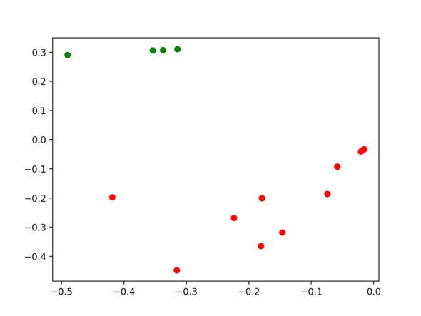
Finally, let’s determine our clusters! The eigenvector row at index i corresponds to the graph node node at index i. From here, the final step is to run a compactness-based clustering algorithm (we’ll use k-means) on the points generated by the rows of eigenvectors. Then, we just map the results back to our original dataset.
from sklearn.cluster import KMeans

def find_clusters(graph, points):
    eigs = laplacian_eigenvectors(graph)
    kmeans = KMeans(n_clusters=2, random_state=0).fit(eigs)
    for i in range(len(kmeans.labels_)):
        if kmeans.labels_[i] == 0:
            points[i].color = "green"
        else:
            points[i].color = "red"
Spectral Clustering Takeaways
We’ve officially just gone through the process of spectral clustering!
The algorithm has some benefits and drawbacks. Defining our own similarity metric allows spectral clustering in various use cases such as image recognition or movie recommendation. On the downside, it can be computationally expensive for large datasets due to O(N²) similarity computations. Additionally, unlike mean-shift clustering, you have to pre-define your k value for how many sections you want to partition your data into.
The source code for this example is posted here.