Basic Machine Learning with KNN and Racket

The web is allowing us to obtain an enormous amount of data about our behavior, which raises an interesting question: how do we manage and use it? One way is with intelligent algorithms, which are being used to bring us ad targeting, recommendation engines, and spam detection, among others.

In this post, I’ll show you how to implement the K Nearest Neighbor (KNN) algorithm in Racket, a dialect of Scheme. Don’t worry, even though some algorithms have roots in neuroscience, machine learning will not make your computer self aware.

Machine Learning with K Nearest Neighbor

KNN is a machine learning classification algorithm that’s lazy (it defers computation until classification is needed) and supervised (it is provided an initial set of training data with class labels). KNN is a simple, easy-to-understand algorithm and requires no prior knowledge of statistics.

The basic premise of KNN is simplistic and reasonable: given an instance of data, look for the k closest neighboring instances, and choose the most popular class among them.

Although simplistic and easy to implement, KNN is not applicable to all scenarios. Since KNN is a lazy algorithm, it is computationally expensive for data sets with a large number of items. The distance from the instance to be classified to each item in the training set needs to be calculated and then each sorted.

Additionally, since KNN uses a distance formula, patterns with less than 10-15 features are recommended, unless some sort of feature extraction or dimensionality reduction is performed. The distance formulas become meaningless at higher dimensionalities. Principle component analysis or linear discriminant analysis can be used to reduce dimensionality, but they are beyond the scope of this post.

The Iris Data Set

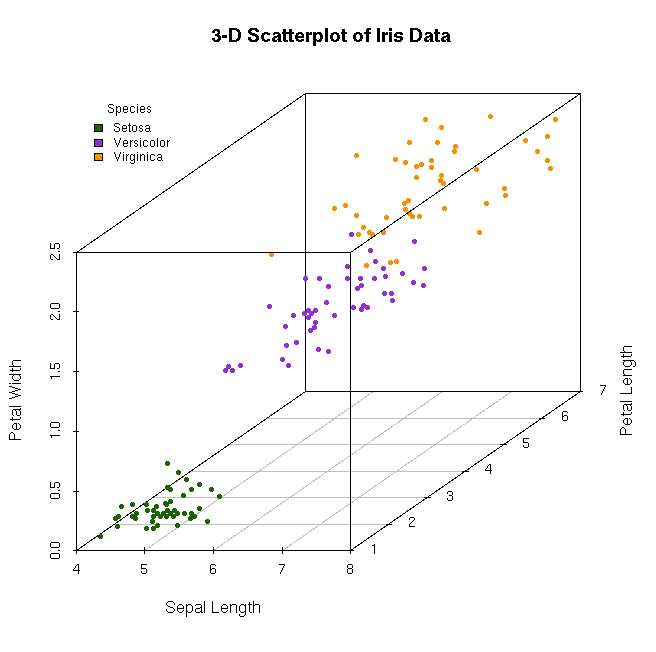
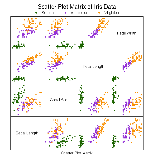
The data set we will be using to test our algorithm is the iris data set. It is a classic multivariate data set used throughout statistics and machine learning. The data set includes 150 instances evenly distributed between 3 species of iris: setosa, virginica, and versicolor. The dataset includes 4 features (properties) for each instance, sepal width, sepal length, petal width, and petal length, as well as a class of which species the instance belongs to. When visually graphed, the iris data is partitioned into 2 distinct clusters. The first cluster is well separated and contains the setosa species. The second cluster contains the virginica and versicolor species.

K Nearest Neighbor in Racket

Racket, formerly known as PLT Scheme, is many things. At its core, it’s is a mutli-paradigm dialect of lisp descending from scheme. At Strange Loop 2012, I had the opportunity to see Matthew Flatt present The Racket Way, and have been looking for a chance to use it since. An implementation of KNN is perfect for this and maps nicely to function composition.

1. Loading the Data

The first task was loading the racket data from a CSV file. I implemented this in a separate package which provides a get-data function. I won’t go over details of implementation here, but the source can be viewed in the racket-knn github repository.

(define training-data (get-data "training.data"))

Results in a list of iris structs.

'(# # # ...)

2. Calculating the Euclidean Distance

The next task was to calculate the euclidean distance from an instance that needs to be classified to each point in our training data. I did briefly experiment with the manhattan distance formula, but it did not perform nearly as well as euclidean distance. The function implementing manhattan distance remains in my code but will not be discussed here.

(define (iris-distance-euclidean from to)
  (let (
        [sld (expt (- (iris-sepal-length from) (iris-sepal-length to)) 2)]
        [swd (expt (- (iris-sepal-width from) (iris-sepal-width to)) 2)]
        [pld (expt (- (iris-petal-length from) (iris-petal-length to)) 2)]
        [pwd (expt (- (iris-petal-width from) (iris-petal-width to)) 2)]
        )

    (cons (sqrt (+ sld swd pld pwd)) (iris-classification to))))

(define classify-me (iris 6.3 2.5 4.9 1.5 "Iris-versicolor"))
(map (curry iris-distance-euclidean classify-me) training-data)

Resulting in a list of pairs, where each pair is defined as (distance . class).

 
'((1.503329637837291 . "Iris-versicolor")
  (2.0371548787463363 . "Iris-versicolor")
  (0.9486832980505138 . "Iris-versicolor")
  (1.1135528725660047 . "Iris-versicolor")
  (0.5 . "Iris-versicolor")
  (1.5427248620541516 . "Iris-versicolor")
  (0.8831760866327849 . "Iris-versicolor")
  (0.948683298050514 . "Iris-versicolor")
  (1.0862780491200221 . "Iris-versicolor") ...)

3. Sorting the Distances & Finding K Neighbor

The next step is to sort the data and take the first k=5 neighbors. We will be building upon the previous chain of expressions.

(define (iris-distance-pair-< i1 i2)
  (< (car i1) (car i2)))

(take 
  (sort 
    (map (curry iris-distance-euclidean classify-me) training-data) 
    iris-distance-pair-<) 
  5)

This results in list of length k=5 of the closest (distance . class) pairs.

'((0.3605551275463984 . "Iris-virginica")
  (0.36055512754639907 . "Iris-virginica")
  (0.41231056256176585 . "Iris-virginica")
  (0.4242640687119282 . "Iris-versicolor")
  (0.43588989435406705 . "Iris-virginica"))

4. Counting the Classes

In preparation for the next step, I defined two helper functions: unique-classes, which returns a unique set of all the classes; and pair-cdr-is?, which makes comparisons a little nicer looking when composed.

(define (unique-classes distance-pairs)
  (list->set (map cdr distance-pairs)))

(define (pair-cdr-is? x pair)
  (equal? (cdr pair) x))

Counting and finding the most popular class among the k=5 nearest neighbors seems easy on paper, but was a bit of a puzzle for me when it came to implementation. My solution was to find the unique set of species classes, count them as they occur in the (distance . class) pair list, and return a new list of (count . class) pairs.

(define (count-all-classes distance-pairs)
  (define (_count-all classes accum)
    (if (set-empty? classes)
      accum
      (_count-all
        (set-rest classes)
        (cons
          (cons (count (curry pair-cdr-is? (set-first classes)) distance-pairs) (set-first classes))
          accum)
        )
      )
    )

  (_count-all (unique-classes distance-pairs) (list))
)

(count-all-classes k-neighbors)

This results in the given list of pairs for our test instance.

'((1 . "Iris-versicolor") (4 . "Iris-virginica"))

5. Sorting & Getting the Most Popular Class

The next step is to sort it in descending order and take the first pair's second element to get the class. The previous expression is expanded upon.

(cdar (sort (count-all-classes k-neighbors) iris-distance-pair->))

Which results in our class predicted by the KNN algorithm.

"Iris-virginica"

Accuracy of Test Data Classifications

When applying the KNN algorithm to a set of test data:

(define k 5)
(define test-data (get-data "test-data/test_data2.csv"))
(define ml-classes (map (curry knn-classify k training-data) test-data))
(define real-classes (map iris-classification test-data))

(pretty-print '("Classified . Actual"))
(map (compose pretty-print cons) ml-classes real-classes)

We can see that the resulting classifications are quite accurate.

'("Classified . Actual")
'("Iris-setosa" . "Iris-setosa")
'("Iris-setosa" . "Iris-setosa")
'("Iris-setosa" . "Iris-setosa")
'("Iris-setosa" . "Iris-setosa")
'("Iris-setosa" . "Iris-setosa")
'("Iris-versicolor" . "Iris-versicolor")
'("Iris-versicolor" . "Iris-versicolor")
'("Iris-versicolor" . "Iris-versicolor")
'("Iris-virginica" . "Iris-versicolor")
'("Iris-versicolor" . "Iris-versicolor")
'("Iris-versicolor" . "Iris-virginica")
'("Iris-virginica" . "Iris-virginica")
'("Iris-virginica" . "Iris-virginica")
'("Iris-virginica" . "Iris-virginica")
'("Iris-virginica" . "Iris-virginica")

Setosa results in 5/5 being classified correctly. Virginica and versicolor result in 4/5 being classified correctly. These result aren't surprising given the scatter plots for the data showing the 2 clusters.

Project Code

All racket code used for this post can be found on github in my racket-knn project. Also included is the R for generating the diagrams and the orange data mining model for random data sampling.