Article summary
Gradient descent is one of those “greatest hits” algorithms that can offer a new perspective for solving problems. Unfortunately, it’s rarely taught in undergraduate computer science programs. In this post I’ll give an introduction to the gradient descent algorithm, and walk through an example that demonstrates how gradient descent can be used to solve machine learning problems such as linear regression.
At a theoretical level, gradient descent is an algorithm that minimizes functions. Given a function defined by a set of parameters, gradient descent starts with an initial set of parameter values and iteratively moves toward a set of parameter values that minimize the function. This iterative minimization is achieved using calculus, taking steps in the negative direction of the function gradient.
It’s sometimes difficult to see how this mathematical explanation translates into a practical setting, so it’s helpful to look at an example. The canonical example when explaining gradient descent is linear regression.
Code for this example can be found here
Linear Regression Example
Simply stated, the goal of linear regression is to fit a line to a set of points. Consider the following data.
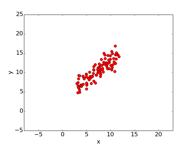
Let’s suppose we want to model the above set of points with a line. To do this we’ll use the standard y = mx + b line equation where m is the line’s slope and b is the line’s y-intercept. To find the best line for our data, we need to find the best set of slope m and y-intercept b values.
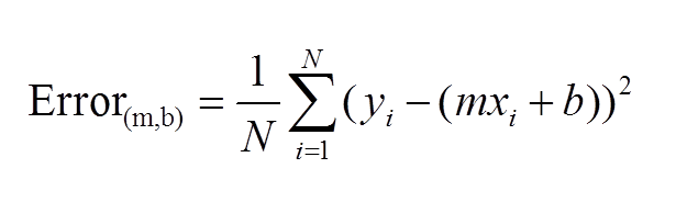
A standard approach to solving this type of problem is to define an error function (also called a cost function) that measures how “good” a given line is. This function will take in a (m,b) pair and return an error value based on how well the line fits our data. To compute this error for a given line, we’ll iterate through each (x,y) point in our data set and sum the square distances between each point’s y value and the candidate line’s y value (computed at mx + b). It’s conventional to square this distance to ensure that it is positive and to make our error function differentiable. In python, computing the error for a given line will look like:
# y = mx + b

# m is slope, b is y-intercept

def computeErrorForLineGivenPoints(b, m, points):

    totalError = 0

    for i in range(0, len(points)):

        totalError += (points[i].y - (m * points[i].x + b)) ** 2

    return totalError / float(len(points))
Formally, this error function looks like:
Lines that fit our data better (where better is defined by our error function) will result in lower error values. If we minimize this function, we will get the best line for our data. Since our error function consists of two parameters (m and b) we can visualize it as a two-dimensional surface. This is what it looks like for our data set:
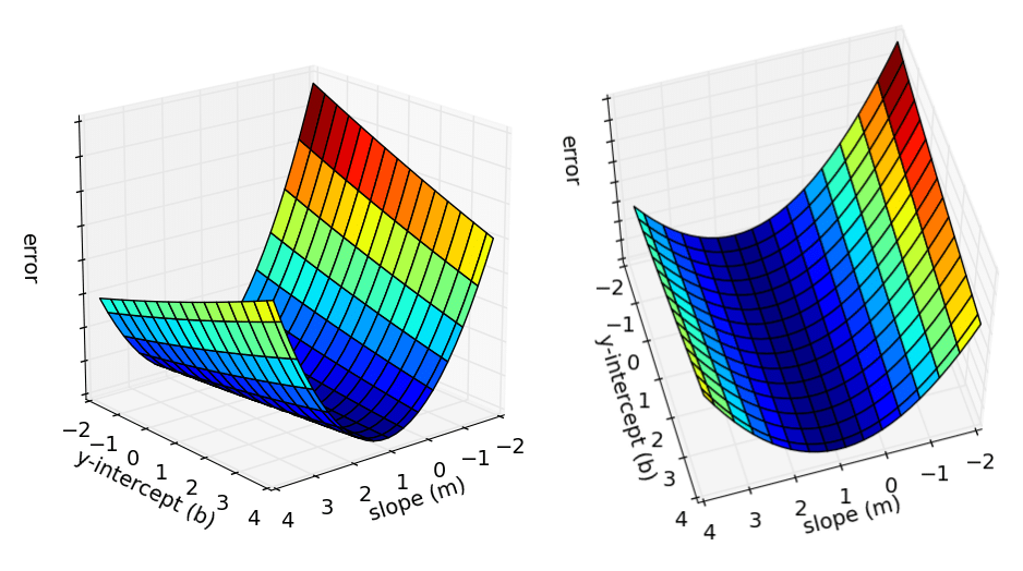
Each point in this two-dimensional space represents a line. The height of the function at each point is the error value for that line. You can see that some lines yield smaller error values than others (i.e., fit our data better). When we run gradient descent search, we will start from some location on this surface and move downhill to find the line with the lowest error.
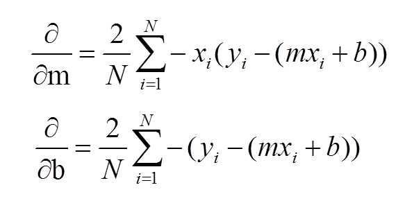
To run gradient descent on this error function, we first need to compute its gradient. The gradient will act like a compass and always point us downhill. To compute it, we will need to differentiate our error function. Since our function is defined by two parameters (m and b), we will need to compute a partial derivative for each. These derivatives work out to be:
We now have all the tools needed to run gradient descent. We can initialize our search to start at any pair of m and b values (i.e., any line) and let the gradient descent algorithm march downhill on our error function towards the best line. Each iteration will update m and b to a line that yields slightly lower error than the previous iteration. The direction to move in for each iteration is calculated using the two partial derivatives from above and looks like this:
def stepGradient(b_current, m_current, points, learningRate):

    b_gradient = 0

    m_gradient = 0

    N = float(len(points))

    for i in range(0, len(points)):

        b_gradient += -(2/N) * (points[i].y - ((m_current*points[i].x) + b_current))

        m_gradient += -(2/N) * points[i].x * (points[i].y - ((m_current * points[i].x) + b_current))

    new_b = b_current - (learningRate * b_gradient)

    new_m = m_current - (learningRate * m_gradient)

    return [new_b, new_m]
The learningRate variable controls how large of a step we take downhill during each iteration. If we take too large of a step, we may step over the minimum. However, if we take small steps, it will require many iterations to arrive at the minimum.
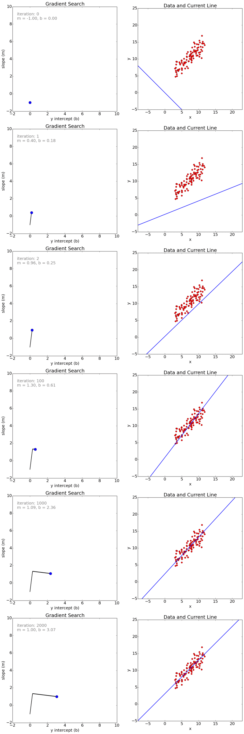
Below are some snapshots of gradient descent running for 2000 iterations for our example problem. We start out at point m = -1 b = 0. Each iteration m and b are updated to values that yield slightly lower error than the previous iteration. The left plot displays the current location of the gradient descent search (blue dot) and the path taken to get there (black line). The right plot displays the corresponding line for the current search location. Eventually we ended up with a pretty accurate fit.
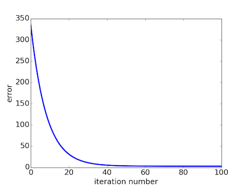
We can also observe how the error changes as we move toward the minimum. A good way to ensure that gradient descent is working correctly is to make sure that the error decreases for each iteration. Below is a plot of error values for the first 100 iterations of the above gradient search.
We’ve now seen how gradient descent can be applied to solve a linear regression problem. While the model in our example was a line, the concept of minimizing a cost function to tune parameters also applies to regression problems that use higher order polynomials and other problems found around the machine learning world.
While we were able to scratch the surface for learning gradient descent, there are several additional concepts that are good to be aware of that we weren’t able to discuss. A few of these include:
- Convexity – In our linear regression problem, there was only one minimum. Our error surface was convex. Regardless of where we started, we would eventually arrive at the absolute minimum. In general, this need not be the case. It’s possible to have a problem with local minima that a gradient search can get stuck in. There are several approaches to mitigate this (e.g., stochastic gradient search).
- Performance – We used vanilla gradient descent with a learning rate of 0.0005 in the above example, and ran it for 2000 iterations. There are approaches such a line search, that can reduce the number of iterations required. For the above example, line search reduces the number of iterations to arrive at a reasonable solution from several thousand to around 50.
- Convergence – We didn’t talk about how to determine when the search finds a solution. This is typically done by looking for small changes in error iteration-to-iteration (e.g., where the gradient is near zero).
For more information about gradient descent, linear regression, and other machine learning topics, I would strongly recommend Andrew Ng’s machine learning course on Coursera.
Example Code
Example code for the problem described above can be found here
Edit: I chose to use linear regression example above for simplicity. We used gradient descent to iteratively estimate m and b, however we could have also solved for them directly. My intention was to illustrate how gradient descent can be used to iteratively estimate/tune parameters, as this is required for many different problems in machine learning.
Maybe I’m missing something, but the y-intercept,slope points plotted in the “Gradient Search” graphs don’t seem to correspond to the blue lines being generated in the “Data and Current Line” graphs. The values for slope seem accurate but the y-intercepts seem off.
Hi Chris, thanks for the comment. The origin (0,0) doesn’t correspond to the bottom left of the plot (rather it’s one tick in on each axis) so it might be a little confusing to read. What specifically looks off?
Hi Matt,
about Chris’s comment:
Look at the fift image: The y-intercept in the left graph (about 2.2) doesn’t correspond with the y-intercept in the right graph (about -8).
Best,
jalil
the y-intercept in the right graph is not -8. For the y-intercept, you need to find the position where x=0.
hie sir, where should i run this project, i mean in centos
This is very interesting. As I don’t have a comp sci background, can you explain when you would use gradient descent to solve a linear regression problem vs. using OLS? Thanks.
Hi Ji-A. I used a simple linear regression example in this post for simplicity. As you alluded to, the example in the post has a closed form solution that can be solved easily, so I wouldn’t use gradient descent to solve such a simplistic linear regression problem. However, gradient descent and the concept of parameter optimization/tuning is found all over the machine learning world, so I wanted to present it in a way that was easy to understand. In practice, my understanding is that gradient descent becomes more useful in the following scenarios:
1) As the number of parameters you need to solve for grows. In our example we had two parameters (m and b). In Andrew Ng’s Machine Learning class on Coursera, he suggests that when you have more than 10,000 parameters gradient descent may be a better solution than the normal equation closed form solution. See the video here: https://www.youtube.com/watch?v=B3vseKmgi8E&feature=youtu.be&t=11m27s
2) When your system of equations is non-linear. Logistic regression (a common machine learning classification method) is an example of this.
3) When an approximate answer is “good enough”.
Thanks for the information! I knew there were nuances I was missing.
I did check on the internet so many times to find a way of applying the gradient descent and optimizing the coefficient on logistic regression the way u did explain it here. I’d like to see another work for you explaining this or if you have any other link
Dear Matt:
I ran your simulation (m=-1, b=0, with 2000 iterations), but the final slope and intercept were not the same as the ones you listed. Also, I ran my own best fit and it matches what you have graphically. Anyway, I am just trying to get the best fit line from your gradient algorithm. Maybe I am missing something??
Dave Paper
I think I have got it now. I was able to create a ‘best fit’ line with the final slope and intercept (from your gradient descent algorithm) that matched the ‘best line’ fit from running numpy ‘polyfit’. Thx for the great example!
dave
Hello, what improvements did you do to the code to match a solution from let’s say, Excel with slope = 1.3224 and interceptio = 7.991? I had to make the code do a lot of iterations to achieve that. Did you managed to do it in 2000 iterations?
Thanks for neatly explaining the concept. One question however, where are you getting the x and y values to compute the totalError and the two new gradients in your code snippets? I can’t figure that out, please help understand.
The x and y values come from the points (e.g., the data set). The points are iterated over and each point (e.g., (x, y) pair) contributes toward the totalError and gradient values.
sometime we do gradient descent and optimization based on each single vector like the case in NN. how would you explain this.
1) Crystal clear. I have one doubt , if the error surface is having only one local minimum(absolute minimum) , then we can set derivation equal to zero (which is nothing but solving simultaneous equations right ? The solution we get from this method will be unique , in this case we no need to worry about GD algo and number of iterations),
2) But in real time we dont know the error surface will have how many locals ( let say if we have m local minimas , all these places will have gradient value will be zeros) . In the iterative process (GD algo), when we near to any of local minima we will stop (again , to reach such any one of local minima will take many number of iterations , is that right ?)
3) As you mentioned is that always right the ‘total error in previous iteration should have lesser than current iteration (It may fluctuate , It depends on learning param ?)’
– your post is too good
Hi Naresh,
Question 1 – Yes, that is correct. We could solve directly for it (as we have two equations, two unknowns, etc.). I chose a simple example to explain the gradient descent idea/concept. However, you could have a problem where you can’t solve for it directly or the cost of doing so is high (see my reply above to Ji-A).
Question 2 – Yes, that is also correct. It’s possible to get suck in local minima. Typically you can use a stochastic approach to mitigate this where you run many searches from many initial states and choose the best result amongst all of them.
Question 3 – In general, the error should always monotonically decrease (if you are truly moving downhill in the direction of the negative gradient). However, depending on your parameter selection (e.g., learning rate, etc.) it is possible to diverge.
Hope that helps.
In OLS cost function (J(theta)) you don’t have to worry about local minimum issues. That is exactly the reason we use convex function to derive it.
Also want to understand how the differentiation is always arriving at a descent.
Vinsent, gradient descent is able to always move downhill because it uses calculus to compute the slope of the error surface at each iteration.
It is my understanding that the gradient of a function at a point A evaluated at that point points in the direction of greatest increase. If you take the negative of that gradient you get the direction of greatest decrease. The gradient vector is derived from the several partial derivatives of the function with respect to its variables. This is why differentiation leads to the direction of greatest descent.
Keeping this in mind, if you are given an error function; by finding the gradient of that function and taking its negative you get the direction in which you have to “move” to decrease your error.
Hope this makes sense.
It’s nice article but I have question to choose m value what should be ideal m value I am working similar Algorithm but not able to solve it.
In my example above m was a parameter (the line’s slope) that we are trying to solve for. So we choose a random initial m value and gradient descent updates it each iteration with a slightly better value until it arrives at the best value (or get’s stuck in a local minimum).
Just pasting my question here : http://stackoverflow.com/questions/26314066/intersection-of-curve-and-find-x-y-point-using-x-and-y-data-point
Thanks, I appreciate your help.
hi, i tried to use the code in your post but however find it not converging somehow. do you know why?
http://nbviewer.ipython.org/github/tikazyq/stuff/blob/master/grad_descent.ipynb
Try using a smaller learning rate. I ran your code with a learning rate of 0.0001 and it seemed to be converging.
Fantastic article!
Very well crafted.
Thank you.
Hi, thanks for the article.
Do you, by any chance, have the original points to test the methods.
Thanks
Very clear example! Could you tell what kind of data structure the ‘points’ variable is? I can’t figure it out. Looks like an array of Point classes, since you use the [] notation to access a point and the dot notation to access x and y of a point.
Points is a list of Point objects (e.g., a class with an x and y property).
Is there somewhere that we can see the whole code example? The snippets are helpful but not entirely sufficient.
Thanks!
Thanks for the comment. I will work to put together a more complete code example and share it.
I have put together an example here: https://github.com/mattnedrich/GradientDescentExample
How do i use this code to find value of Y for a new value of x?
Nicely explained!! Enjoyed the post.Thanks
That was such an awesome explanation !! Can you also explain logistic regression and gradient descent
Thanks Praveen, glad you liked it. Also, thanks for the logistic regression suggestion, I may consider writing a post on that in the future.
Matt, this is a boss-level post. Really helped me understand the concept. Gold stars and back-pats all round.
I really liked the post and the work that you’ve put in. I suggest you add a like button to your posts.
Hi Matt,
Overall your article is very clear, but I want to clarify one important moment. The real m and b are 1.28 and 9.9 respectively for the data you ran on your code (e.g. data.csv). But your code gives us totally different results, why is that?
I know we can get that true result above by giving different random m and b, but shouldn’t our code work for any random m and b?
Would be kind clarifying that moment please, it is very important for me.
Thank you in advance.
Hi Altay, how are you computing 1.28 and 9.9 for the real m and b?
Hi,
I’ve just simply used excel to compute that linear regression. Also vusualized that line graphically to check.
It’s important to understand that there is no “true” or “correct” answer (e.g., m and b values). We are trying to model data using a line, and scoring how well the model does by defining an objective function (error function) to minimize. It’s very possible that Excel is using a different objective function than I used. It’s also possible that I did not run gradient descent for enough iterations, and the error difference between my answer and the excel answer is very small. Ideally, you would have some test data that you could score different models against to determine which approach produces the best result.
Hi Matt,
Sorry for my late reply.
But I thought that Gradient Descent should give us the exact and most optimal fitting m and b for training data, at least because we have only one independent variable X in the example you gave us.
If I miss smth, correct me please.
If you compare the error for the (m,b) result I got above after 2000 iterations, it is slightly larger than the (m,b) example you reported from excel (call the compute_error_for_line_given_points function in my code with the two lines and compare the result). Had I ran it for more than 2000 iterations it would have eventually converged at the line you posted above.
What I was trying to say above is that gradient descent will in theory give us the most optimal fitting for m and b for a defined objective function. Of course, this comes with all sorts of caveats (e.g., how searchable is the space, are there local minima, etc.).
I am terribly sorry Matt, but there was a slight error with data selection when I was creating my regression formula in excel, so I corrected it and results are m = 1.32 and b = 7.9. And this result is achieved using your python code when I gave m = 2 and b = 8 as initial parameters.
And I played with some other different values as an initial m and b and number of iterations, after which I realized that the best starting values were m = 2 and b = 8.
And I made conclusion that the main point is to give right starting m and b which I do not know how to do.
So I want to thank you for your your article and your replies to my comments which was a sort of short discussion.
Assuming it is the true minimum, it should eventually converge to (1.32, 7.9) regardless of what initial (m,b) value you use. It may take a very long time to do so however.
In the error surface above you can see a long blue ridge (near the bottom of the function). My guess is that the search moves into this ridge pretty quickly but then moves slowly after that. My guess is that you just aren’t running it long enough if you are getting different results for different starting values.
Hi Matt,
Thank you once again. I got correct results just by increasing number of iterations to 1000000 and more.
Hi Matt.
Thanks for efforts. I’m trying to refresh my knowledge with your article.
Can you please explain what do you mean by “Each point in this two-dimensional space represents a line. The height of the function at each point is the error value for that line.” Does that mean each point IS line or what? I cant understand.
Thanks
I am also confused by this point / line vocabulary here. Too bad you did not get any answer.
I believe the 2 dimensions in this 2-dimensional space are m (slope of the line) and b (the y-intercept of the line). Therefore any point in the m,b space will map into a line in the x-y space. I suppose Matt added the 3rd dimension to the m,b space by showing the error associated with the line associated with the m,b pair.
Matt,
Thanks for your blog, especially using PDE and converting into function is quite useful. BTW, this is quite useful for people who is taking CS.190.x on EDX.
Cheers
Hey Matt, just wanted to say a huge “THANK YOU!!” this is the best simple explanation of linear regression + gradient on the Web so far.
Hi, Matt
can you please give an example or an explanation og how gradient descent helps or works in text classification problems.
Hi, this is really interesting, could you also make an article about stochastic gradient descent, please. Thanks.
Matthew,
What is the license for your code examples?
@Michael – great question, I’ve added an MIT license.
Is gradient descent algorithm applied in hadoop….if so how ??
can you explain more about defferentiating the error function specifically?
hi
is there any body who knows some information about shape topology optimization by phase field method ?
best regards
thanks for your web and reply
I’m beginning to study data science and this blog is very helpful. Thanks Matt. Just one question, could you explain how you derive the partial derivative for m and b? thanks a lot.
Can only say: fantastic !!!
Thankyou. I’ve never seen a better explanation in any of my class (I’m a UG Bioinformatics student struggling to understand such concepts) and now I understand this concept thoroughly.
Excellent explanation.
Are you using this to spot a trend in a stock? I have coded something in easy language for Trade Station and what I have found is that there is no correct chart size for the day.
In other words no matter what chart size I use I will know if I should be a buyer or a seller based on the trend for the day.
I then take a measurement and can make a logical decision about what the big boys are doing and then I do what they do.
For instance……I was 100 percent sure that buying EMINI’s above 2060 was a terrible decision and I had calculated that the stall out was going to be 2063.50 …
I also was a seller of oil futures above 42.76 and then I hit it again on the retrace above 42.40.
Are you interested in this type of thing or is this outside the realm of what you are doing?
Great post! I’m trying to understand the type of math behind neural networks through examples and this helped a whole bunch! I did my own implementation of your code in Google Spreadsheets/Google Script (7.5MB GIF) http://i.imgur.com/KcgisHN
Hello,
Thanks for the explanation. Does the error function remain same for exponential curve i.e (y – w * e^(lambda * x))^2? If not how does it change when I try to fit a curve using exponential curve and similarly for a hypo exponential – convolution of exponential’s. I am trying to fit curve which is a probability density function using exponential PDF.
To start with I am trying single exponential curve.
I tried implementing the same algorithm for exponential curve but it doesn’t work. The matlab code for the same can be found here – http://pastebin.com/LvASET0p
Thanks for writing this! I’m actually taking Andrew Ng’s MOOC, and I was looking for an explanation of gradient descent that would go into a little more detail than he gave (at least initially…I haven’t finished the course) and show me visually what gradient descent looked like and what the graph for the error function looked like. Your explanation was really helpful and helped me picture what was going on. Thanks!
Me too. I studied regression analysis once a long time ago but I could not recall the details. I searched a lot of other websites and I could not find the explanation that I needed there either. Oddly, conventional presentations of elementary machine learning methods seem to have a meta-language that is half way between mathematics and programming that are riddled with little but significant explanatory gaps.Some details are so important that they should be pointed out in order to make a consistent presentation.
Awesome! Thank you.
At my current job we are using this algorithm specifically. without your example, I would not have been able to figure it out so easily.
What I am trying to figure out is what would be a good way to generate example data for a multi-point(x, y, z) approach using a quadratic in three dimensions?
Matt, This is the best and the most practical explanation of this algorithm. Kudos!! Thanks a lot.
Awesome article………. I was trying to get my head around Neural Networks and came through Gradient Descent……of all article I searched this is the most well explained Article. Thanks a ton.
On a lighter note there is a saying “You do not really understand something unless you can explain it to your grandmother.”…….Well now I can explain my grandmother this stuff :D
Thank you for this valuable article.
I have a problem with my code, I’m using (Simple Regression Problem//
F(a)= a^4+ a^3+ a^2+ a)
but there is no convergence
its about Cartesian genetic programming
my question is
should i use the gradient with it to solve the problem or?????
thanks
Thank you. All i every well detailed but one “line” has no explanation, and this is ( to me the core of the algorithm):
Why on each iteration do you determine that
new_b = b_current – (learningRate * b_gradient)
( same for m : why is the new value = the old value minus the new calculated one )
or, to use your wording: why is this meaning going downhill ?
Thanks for such an fantastic article.
I am attending online course of Prof. Andrew Ng from Coursera.
Your article has contributed to remove many confusions.
In your example I could not find where you are using “learning rate”?
Where you use 0.0001 ?
Thanks in advance for reply.
Bharat.
hello sir, i want to know that if i am training one robot that identify handwitten alphabet character and if i am giving training of character ‘A’ , 50 different training latter A given to robot. then here gradient descent is used or any other?
Can you share the code to generate the gif? Did you just call the matplot lib everytime you compute the values of intercept and slope? I don’t seem to find it on the GitHub
Hello,
In statistics, we use the “Centroid” point to fix at least a point of the line ” Y=m X + b.
very useful, after with only one other point we have the full equation.
(see linear regression in statistics)
But I see in machine learning that you jump to Cost Fonction type of problem to minimize.
and yes, it has to search for both m, and B, the slope and the “Bias” in same time.
Would you please help, explain why they don’t use CENTROID methode ?
thanks
does it work for multi linear regression? if it does, can you please show me how it works? thanks
I am confused in one thing. We have to take the partial derivative of the cost function continuously again and again until we get the local minimum or the derivative will be taken only once?
Is it that once we get the equations
b_gradient += -(2/N) * (points[i].y – ((m_current*points[i].x) + b_current))
m_gradient += -(2/N) * points[i].x * (points[i].y – ((m_current * points[i].x) + b_current))
by taking the partial derivative once and then it will calculate the parameters by itself each time in a loop?
I hope you understand my question..
thanks
Hi Matt:
When I run your code with initial m = -1 and b = 2 for 2000 iterations, I get the following:
b = 0.0607
m = 1.478
When I use polyfit and lineregress functions, I get the following:
b = 7.99
m = 1.322
I believe that I am running your code correctly. Maybe I am doing something wrong??
dave
awesome explanation.
thanks so much
Thanks for the post Matt.. very well explained.
Amazing post. Exactly what I needed to get started. This beautiful explanation of yours give a feel of the mathematics and logic behind the machine learning concept.
Thanks,
Khalid
Hello,
Very Nicely written.
Thank You for this.
Just Curious–Do you have a similar example for a logistic regression model?
If not- Then Can you please share a similar example for logistic regression.
Thank You Again.
hello
can anyone help me
how can i run this in eclipse
Hi Matt, Thanks for this tutorial. I have been searching for clear and consice explanation to machine learning for a while until I read your article. The animation is great and the explanation is excellent. After reading through it I have managed to replicate it with your data set using T-SQL.I am.over the moon.and so grateful to you for making me understand the concepts of gradient descent. If you do have any other machine learning tutorials kindly send me the links in your response.Thanks
Michael
Hey Matt,
Sorry if I am repeating a question. I havent read all the comments but how do you come up with the value learningRate? is it Hit and trial?
Yes, it’s largely trial and error. Plotting the error after each iteration can help you visualize how the search is converging – check out this SO post http://stackoverflow.com/questions/16640470/how-to-determine-the-learning-rate-and-the-variance-in-a-gradient-descent-algori
Great explanation! Thanks a lot.
Awesome .
Please include an article for stochastic gradient too .
A very good introduction. Covers the essential basics and gives just about enough explantion to understand the concepts well.
One quick question. Apologies if this is a repeat!
You did mention that there can be situations in which we might be stuck in a “Local Minima” & to resolve this we can use “Stochastic Gradient Descent”. But, how do we realize OR understand in the first place, that we are stuck at a local minima and have not already reached the best fitting line?
why do u increment the gradient?
is there someone to let me know what this X is for… in 2nd equation????
why is not it in other equation:
b_gradient += -(2/N) * (y – (m*x) + b))
m_gradient += -(2/N) * x * (y – ((m*x) + b)
i am talking about the x over this dotted place
-(2/N)*……………*(y – ((m * x) + b))
Thanks for the very clear example of linear regression. I’d like to do the surface plot shown just below the error function using matplotlib. I’m having a lot of trouble. I wonder if anyone else has tried this or if Matt is still reading comments.
-2/N should be put out of the for loop right ?
Exactly my thought, but you havent got response, I the -2/N part should go outside the loop too
I am facing problem with a particular data-set even with your python example:
2104,400
1600,330
2400,369
1416,232
3000,540
def computeErrorForLineGivenPoints(b, m, points):
totalError = 0
for i in range(0, len(points)):
totalError += (points[i].y – (m * points[i].x + b)) ** 2
return totalError / float(len(points))
in the above code, for the function “computeErrorForLineGivenPoints(b, m, points)”, what are the parameter values you give for b(y-intercept) and m(slope) parameters. How do you choose b and m ?
I can see from the gradient descent plot that you take only the values between -2 and 4 for both y and m. Why cant it take any other values outside that range ?
The “computeErrorForLineGivenPoints” function is just used to compute an error value for any (m, b) value (i.e., line). I’m using it to show that the error decreases during each iteration of the gradient descent search.
Great page!!! I have one question. How do you put the code in your html? Looks really cool. I want to do the same thing.
Very well written and explained. You inspired me to read and explore more on ML algorithms . Thanks a lot!!!
Clear and well written, however, this is not an introduction to Gradient Descent as the title suggests, it is an introduction tot the USE of gradient descent in linear regression. Gradient descent is not explained, even not what it is. It just states in using gradient descent we take the partial derivatives. The links to Wikipedia are of little use, because these pages are not at all introductory, that’s why I came here. Again, the content is good, but not what it is supposed to be.
Great Explanation!
The only Thing I don’t understand:
Where did you get those Derivatives from?
“These derivatives work out to be:” is not that helpful :(
Thank you very much for fluent and great explanations !!!
At last, I got the Gradient Descent for you.
After a couple of months of studying missing puzzle on Gradient Descent, I got very clear idea from you.
Thanks!!