Mean Shift Clustering

Mean shift clustering is one of my favorite algorithms. It’s a simple and flexible clustering technique that has several nice advantages over other approaches.

In this post I’ll provide an overview of mean shift and discuss some of its strengths and weaknesses. All of the code used in this blog post can be found on github.

Kernel Density Estimation

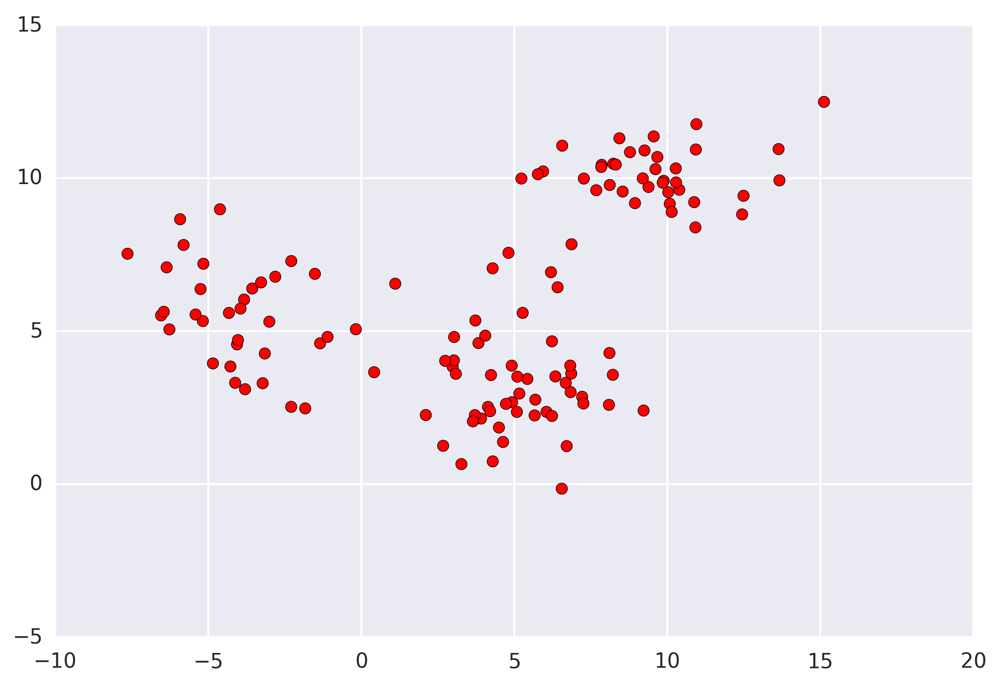
The first step when applying mean shift (and all clustering algorithms) is representing your data in a mathematical manner. For mean shift, this means representing your data as points, such as the set below.

Mean shift builds upon the concept of kernel density estimation (KDE). Imagine that the above data was sampled from a probability distribution. KDE is a method to estimate the underlying distribution (also called the probability density function) for a set of data.

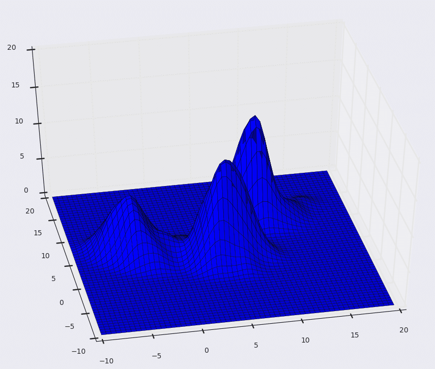
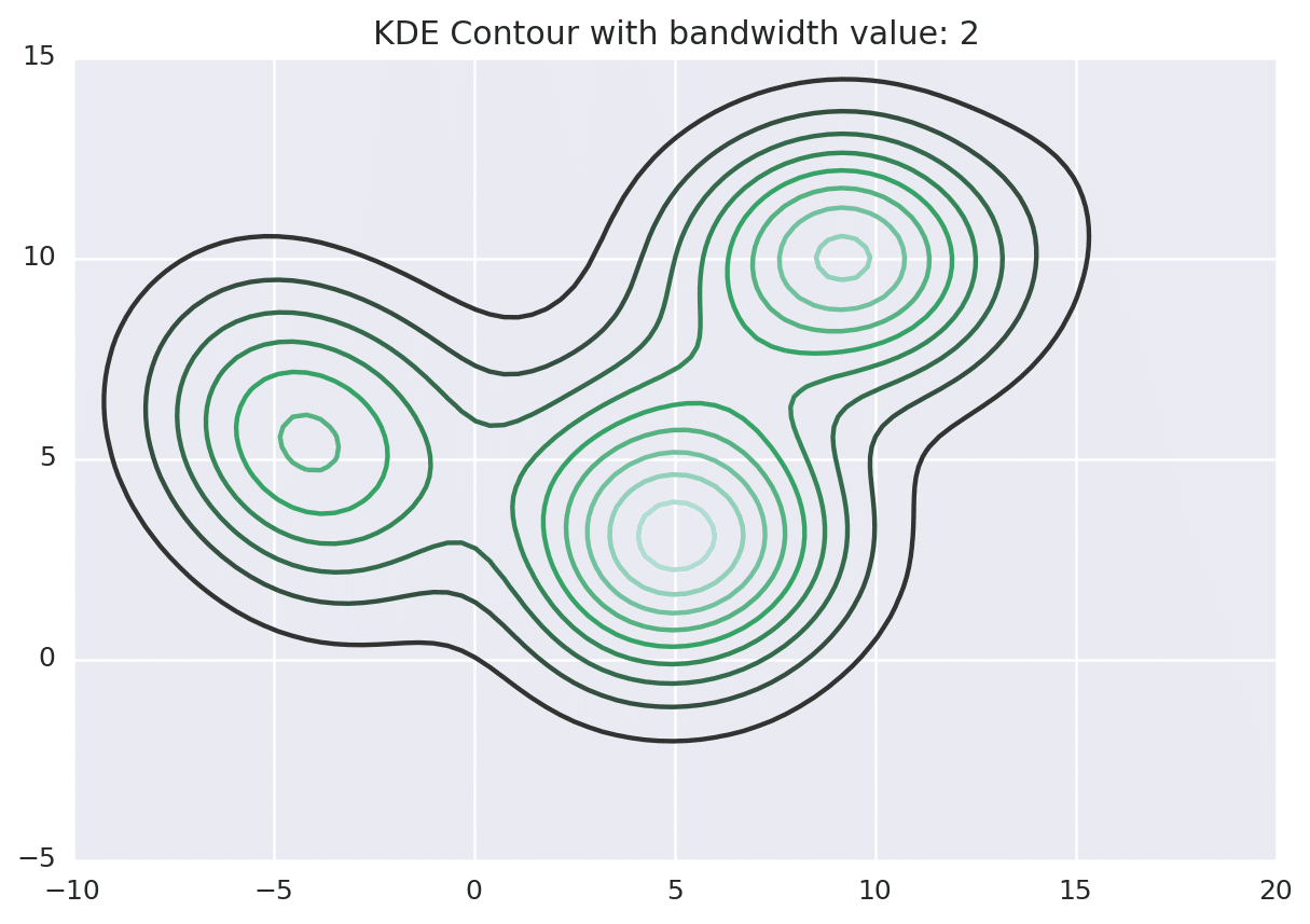
It works by placing a kernel on each point in the data set. A kernel is a fancy mathematical word for a weighting function. There are many different types of kernels, but the most popular one is the Gaussian kernel. Adding all of the individual kernels up generates a probability surface (e.g., density function). Depending on the kernel bandwidth parameter used, the resultant density function will vary.

Below is the KDE surface for our points above using a Gaussian kernel with a kernel bandwidth of 2. The first image is a surface plot, and the second image is a contour plot of the surface.

Mean Shift

So how does mean shift come into the picture? Mean shift exploits this KDE idea by imagining what the points would do if they all climbed up hill to the nearest peak on the KDE surface. It does so by iteratively shifting each point uphill until it reaches a peak.

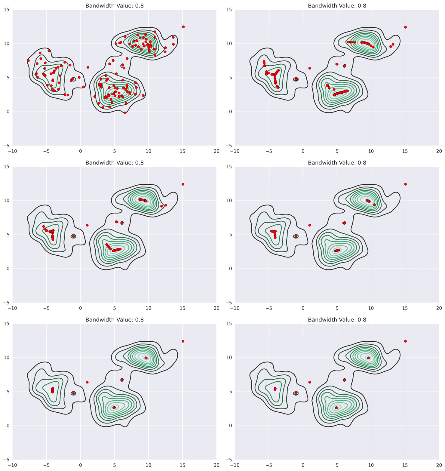
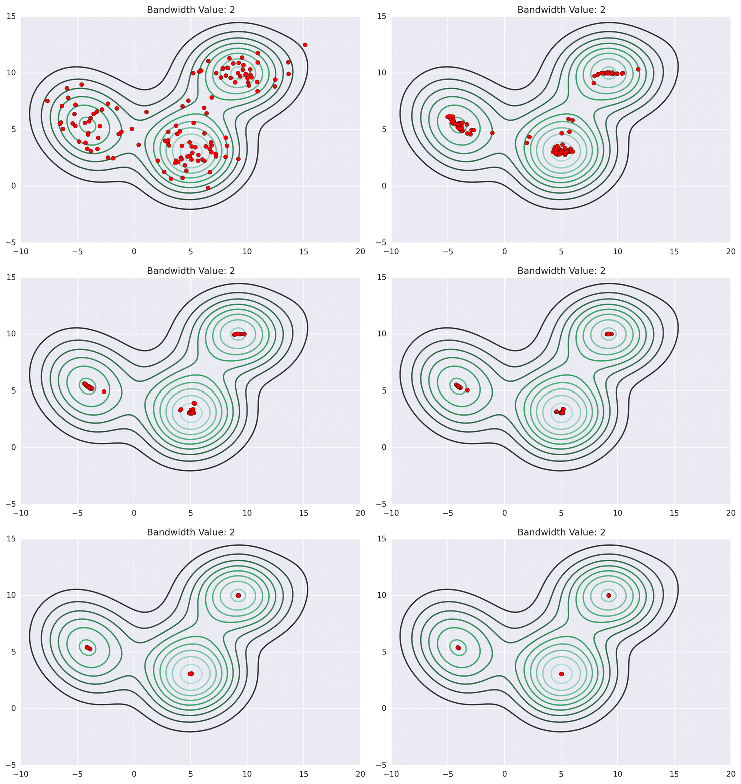
Depending on the kernel bandwidth used, the KDE surface (and end clustering) will be different. As an extreme case, imagine that we use extremely tall skinny kernels (e.g., a small kernel bandwidth). The resultant KDE surface will have a peak for each point. This will result in each point being placed into its own cluster. On the other hand, imagine that we use an extremely short fat kernels (e.g., a large kernel bandwidth). This will result in a wide smooth KDE surface with one peak that all of the points will climb up to, resulting in one cluster. Kernels in between these two extremes will result in nicer clusterings. Below are two animations of mean shift running for different kernel bandwidth values.

The top animation results in three KDE surface peaks, and thus three clusters. The second animation uses a smaller kernel bandwidth, and results in more than three clusters. As with all clustering problems, there is no correct clustering. Rather, correct is usually defined by what seems reasonable given the problem domain and application. Mean shift provides one nice knob (the kernel bandwidth parameter) that can easily be tuned appropriately for different applications.

The Mean Shift Algorithm

As described previously, the mean shift algorithm iteratively shifts each point in the data set until it the top of its nearest KDE surface peak. The algorithm starts by making a copy of the original data set and freezing the original points. The copied points are shifted against the original frozen points.

The general algorithm outline is:

for p in copied_points:

    while not at_kde_peak:

        p = shift(p, original_points)

The shift function looks like this:

def shift(p, original_points):

    shift_x = float(0)

    shift_y = float(0)

    scale_factor = float(0)

    for p_temp in original_points:

        # numerator

        dist = euclidean_dist(p, p_temp)

        weight = kernel(dist, kernel_bandwidth)

        shift_x += p_temp[0] * weight

        shift_y += p_temp[1] * weight

        # denominator

        scale_factor += weight

    shift_x = shift_x / scale_factor

    shift_y = shift_y / scale_factor

    return [shift_x, shift_y]

The shift function is called iteratively for each point, until the point it not shifted by much distance any longer. Each iteration, the point will move more closer to the nearest KDE surface peak.

Image Segmentation Application

A nice visual application of mean shift is image segmentation. The general goal of image segmentation is to partition an image into semantically meaningful regions. This can be accomplished by clustering the pixels in the image. Consider the following photo that I took recently (largely because the nice color variation makes it a nice example image for image segmentation).

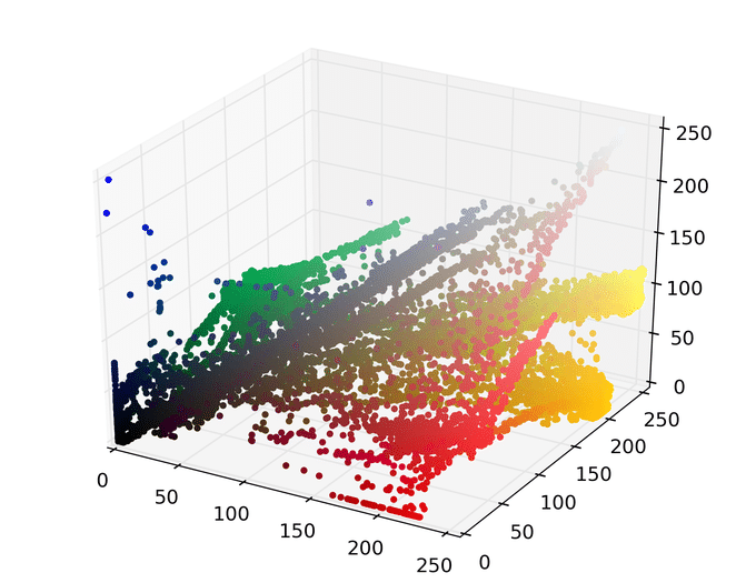
The first step is to represent this image as points in a space. There are several ways to do this, but one easy way is to map each pixel to a point in a three dimensional RGB space using its red, green, and blue pixel values. Doing so for the image above results in the following set of points.

We can then run mean shift on the above points. The following animation shows how each point shifts as the algorithm runs, using a Gaussian kernel with a kernel bandwidth value of 25. Note that I clustered scaled down version of the image (160×120) to allow it run in a reasonable amount of time.

Each point (e.g., pixel) eventually shifted to one of seven modes (e.g., KDE surface peaks). Showing the image using the color of these seven modes produces the following.

Comparison to Other Approaches

As I mentioned above, I really like mean shift because of its simplicity. The entire end result is controlled by one parameter—the kernel bandwidth value. Other clustering approaches, such as k-means, require a number of clusters to be specified as an input. This is acceptable for certain scenarios, but most of the time the number of clusters is not known.

Mean shift cleverly exploits the density of the points in an attempt to generate a reasonable number of clusters. The kernel bandwidth value can often times be chosen based on some domain-specific knowledge. For example, in the above image segmentation example, the bandwidth value can be viewed as how close colors need to be in the RGB color space to be considered related to each other.

Mean shift, however, does come with some disadvantages. The most glaring disadvantage is its slowness. More specifically, it is an N squared algorithm. For problems with many points, it can take a long time to execute. The one silver lining is that, while it is slow, it is also embarrassingly parallelizable, as each point could be shifted in parallel with every other point.