Article summary
In a world full of data that seldom follows nice theoretical distributions, the Central Limit Theorem is a beacon of light. Often referred to as the cornerstone of statistics, it is an important concept to understand when performing any type of data analysis.
Motivation
Suppose that we are interested in estimating the average height among all people. Collecting data for every person in the world is impractical, bordering on impossible. While we can’t obtain a height measurement from everyone in the population, we can still sample some people. The question now becomes, what can we say about the average height of the entire population given a single sample.
The Central Limit Theorem addresses this question exactly. Formally, it states that if we sample from a population using a sufficiently large sample size, the mean of the samples (also known as the sample population) will be normally distributed (assuming true random sampling). What’s especially important is that this will be true regardless of the distribution of the original population.
When I first read this description I did not completely understand what it meant. However, after visualizing a few examples it become more clear. Let’s look at an example of the Central Limit Theorem in action.
Example
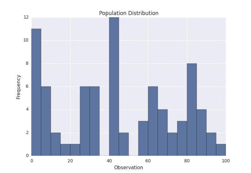
Suppose we have the following population distribution.
I manually generated the above population by choosing numbers between 0 and 100, and plotted it as a histogram. The height of the histogram denotes the frequency of the number in the population. As we can see, the distribution is pretty ugly. It certainly isn’t normal, uniform, or any other commonly known distribution.
In order to sample from the above distribution, we need to define a sample size, referred to as N. This is the number of observations that we will sample at a time. Suppose that we choose N to be 3. This means that we will sample in groups of 3. So for the above population, we might sample groups such as [5, 20, 41], [60, 17, 82], [8, 13, 61], and so on.
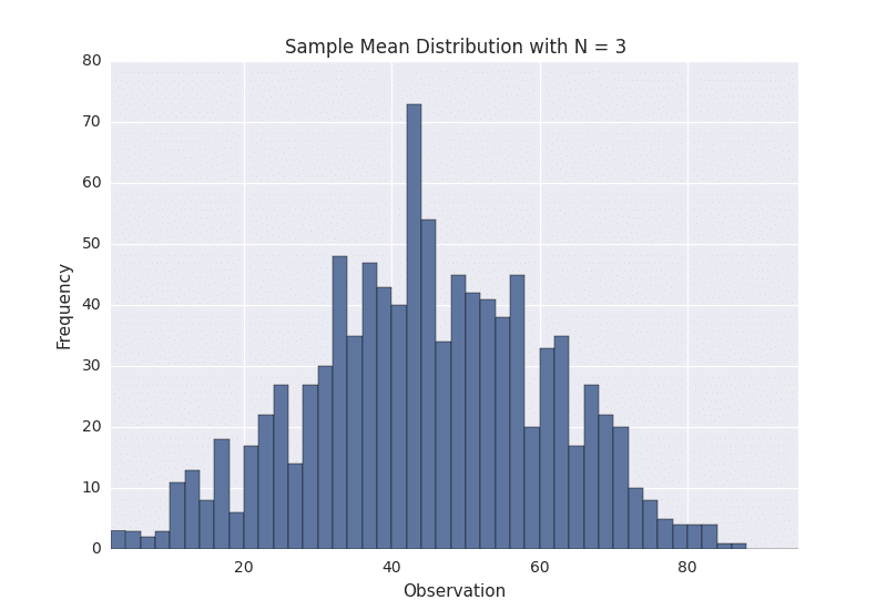
Suppose that we gather 1,000 samples of 3 from the above population. For each sample, we can compute its average. If we do that, we will have 1,000 averages. This set of 1,000 averages is called a sampling distribution, and according to Central Limit Theorem, the sampling distribution will approach a normal distribution as the sample size N used to produce it increases. Here is what our sample distribution looks like for N = 3.
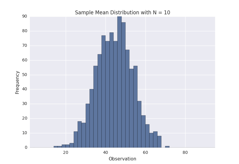
As we can see, it certainly looks uni-modal, though not necessarily normal. If we repeat the same process with a larger sample size, we should see the sampling distribution start to become more normal. Let’s repeat the same process again with N = 10. Here is the sampling distribution for that sample size.
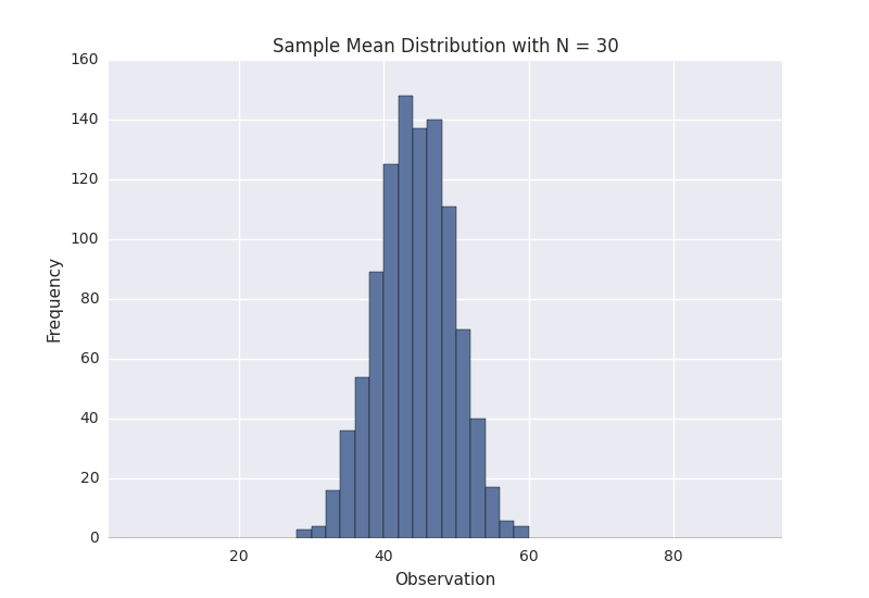
This certainly looks more normal, and if we repeated this process one more time for N = 30 we observe this result.
The above plots demonstrate that as the sample size N is increased, the resultant sample mean distribution becomes more normal. Further, the distribution variance also decreases. Keep in mind that the original population that we are sampling from was that weird ugly distribution above.
Further Intuition
When I first saw an example of the Central Limit Theorem like this, I didn’t really understand why it worked. The best intuition that I have come across involves the example of flipping a coin. Suppose that we have a fair coin and we flip it 100 times. If we observed 48 heads and 52 tails we would probably not be very surprised. Similarly, if we observed 40 heads and 60 tails, we would probably still not be very surprised, though it might seem more rare than the 48/52 scenario. However, if we observed 20 heads and 80 tails we might start to question the fairness of the coin.
This is essentially what the normal-ness of the sample distribution represents. For the coin example, we are likely to get about half heads and half tails. Outcomes farther away from the expected 50/50 result are less likely, and thus less expected. The normal distribution of the sampling distribution captures this concept.
The mean of the sampling distribution will approximate the mean of the true population distribution. Additionally, the variance of the sampling distribution is a function of both the population variance and the sample size used. A larger sample size will produce a smaller sampling distribution variance. This makes intuitive sense, as we are considering more samples when using a larger sample size, and are more likely to get a representative sample of the population. So roughly speaking, if the sample size used is large enough, there is a good chance that it will estimate the population pretty well. Most sources state that for most applications N = 30 is sufficient.
These principles can help us to reason about samples from any population. Depending on the scenario and the information available, the way that it is applied may vary. For example, in some situations we might know the true population mean and variance, which would allow us to compute the variance of any sampling distribution. However, in other situations, such as the original problem we discussed of estimating average human height, we won’t know the true population mean and variance. Understanding the nuances of sampling distributions and the Central Limit Theorem is an essential first step toward talking many of these problems.
Additional Resources
I found the Khan Academy videos on Central Limit Theorem to be especially helpful.
If you would like to play around with sampling distributions, I have put some Central Limit Theorem demo code on GitHub.


Hey this was pretty neat, and really accessible. Cheers!
Thanks, glad you liked it.
Maybe it’s just me, but I always feel that explanations of the CLT do not sufficiently emphasize that it says nothing about any single sample. It says something about the mean of a WHOLE BUNCH of samples. In order to make used of the CLT you have to keep taking samples, and each sample has to be of sufficient size in order for the CLT to hold true. Maybe I’m the only one who ever gets confused about this, but I’m always surprised this isn’t restated a couple of times when explaining the CLT.
Oh, but the CLT *does* say something about a single sample as long as you start talking about the probability of that single sample’s mean — which this explanation failed to get to. The good thing about this explanation and its focus on “a whole bunch of samples” is that we can get an intuition for what the sample mean’s probability distribution looks like by seeing a histogram of many sample means.
Nice. However, the best presentation of the central limit theorem I’ve ever seen was by Brad Osgood during his course on the Fourier transform and its applications [1] and [2]
[1] https://www.youtube.com/watch?v=LA4Uv6PMRTM
[2] http://see.stanford.edu/materials/lsoftaee261/book-fall-07.pdf
Thanks for the feedback, I’ll check out the links.
The video is essential :-) For some reason I think of Osgood as Gilderoy Lockhart with an aptitude for mathematics. I like his way of presenting things, but of course YMMV.
Great. This helped tremendously as I am sampling-plan-challenged. For clarification, I thought N = lot size and n = sample number. In your example you say N= 30 is sufficient. That is lot size and then a sampling from that?
Note: I am using 30 (N) as lot size and plan to test 10 (n) from 3 different lots. Sound right?
Matt,
Good job trying to explain a challenging topic. We provide statistics tutoring to MBA/CFA students and know how challenging this topic is for students to grasp. Although this is almost always covered in all courses, most faculty/students just gloss over this concept even though it is foundational or as you called it a ‘corner stone’ topic.
It will help your readers to understand the term ‘sampling distribution’. And also have some diagram that shows how sampling distributions of different underlying distributions become ‘normally shaped’ as the sample size increases. Happy to assist with this diagram/chart if you think it will be helpful.
Senith
PS: Would be great if you can share an example of how you used the CLT on a project at work. Am sure your readers would love it and we could give our students a current example of the CLT application :)
This is the BEST explanation that I’ve seen thus far. Every explanation that I read said exactly what you said but your example was the only one that helped me get it. THANK YOU!!
Thanks for the comment, glad you liked it.
That’s a pretty awesome article, i was so much confused now i am relax. The figures are really helpful and python code. Thanks
Wow!!!Thanx alot…i now understand the concept of Central limit theorem!!
Matt, please humor an old guy for a couple minutes. Most of my encounters with the CLT occurred in Santa Barbara in the late 70’s. Haven’t used it much since then so my memory is a bit hazy. Can’t remember exactly what my girlfriend looked like either. Oh well.
Regarding Mr. Seniths request for a real life example of the CLT in action, it seems to me we used it to determine what sample size was required to produce a number that could be used with a reasonable degree of confidence.. I know that’s kind of restating the question as the answer but it’s my best recollection.
Also, the example which got me over the hump was: “We want to know the average distance between off ramps on an interstate highway.” I’m not sure why but being able to look at it in a linear sort of way made it easier for me to wrap my head around it. That’s all I got. Thanks for a good article and for the walk down memory lane.
Matt:
Thank you for such a nice explanation!
Thanks for the explaination
You have explained the Central Limit Theorem very well. Thanks Matt.
This has made my day thanks from zambia
the mean of the sampling distribution coincides with the unknown mean of the population. if one doesn’t know the standard deviation of the population either, we’ll approximate it with the standard deviation of our first sample. CLT says that if we knew the standard deviation of the population, then the sampling distribution of say a million samples, all of size N=30 (for example), will have a standard deviation = the standard deviation of the population, divided by square root on N. So instead of taking a million samples, we just take one, we calculate its standard deviation and mean, and we know that with probability 95% that our sample’s mean is no further from the true mean of the population, than 2 standard deviations of our unique sample ( with which we approximated the standard deviation of the population) divided by square root on N. Thus the interval [unique sample mean – 2 * unique’s sample standard deviation divided by the size N of our unique sample, unique sample mean + 2 * unique’s sample standard deviation divided by the size N of our unique sample] will capture the true mean of the population in 95% of such one sample trials. So you can build the above confidence interval for the true mean, with the above level of confidence (95%), using just one sample, not a million samples. The entire simplification of evaluating the true mean of the population using just one sample is all due to CLT!
For your example with randomly picked numbers from zero to 100: looking at the histogram, and just counting, it looks like you have 81 numbers total in the population. So, with N=30, you are sampling about 37% of the total population!!
I didn’t bother to calculate the actual population mean, but it looks like it is approx 45 from the N=30 histogram. And yet, from that same histogram I can see that, even when measuring almost 40% of the total population any particular sample of 30 can still be off pretty dramatically. The histogram for N=30 is showing the variance is about +/- 15. So, on any particular sample of 30, even after checking almost 40% of the entire population your answer could still be off by as much as one third: +/- 33%. That’s pretty shocking. Of course, this is just one particular example, and an example deliberately using fairly random data. As you say, the variance would have been much smaller for a less random population distribution.