During my time as an undergraduate research assistant in a biomedical imaging lab, I created a Python script that displays 3D meshes of cancerous tumors using the marching cubes algorithm. Here, I’ll outline how the algorithm works. Then, I’ll show a simple implementation example using the marching_cubes() function from the Python scikit-image library.
Marching Cubes Explained
The marching cubes algorithm takes in a 3D scalar field as input and generates a polygonal mesh from an isosurface.
Definitions
A scalar field is a function that returns a single value for any point in space. For our purposes, we’ll represent it as a 3D array where each index (x, y, z) corresponds to a scalar value. An isosurface is a 3D representation of a surface within a volume of data (e.g. a 3D scalar field) where all points have the same scalar value, referred to as the iso-value. The resulting polygonal mesh is a collection of vertices, edges, and faces that can be used to display a 3D model.
Process
First, the scalar field is split into cubes such that each value at (x, y, z) is the corner of a cube. For the 8 corners of each cube, it compares the 8 scalar values to the iso-value. Each corner is assigned a bit in an integer. If the scalar value is higher than the iso-value, the point is inside the surface, and we set that corner’s bit to 1. If the value is lower, the point is outside the surface, and we set that corner’s bit to 0. The final result of these comparisons is an 8-bit integer (e.g., 01011001).
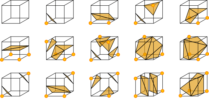
Given that a point can either be 1 or 0 and a cube has 8 corners, there are 2^8 = 256 different configurations. And, each configuration represents a different way the iso-surface intersects the cube. Since there is a set number of configurations, you can precompute them in a triangulation table, which tells us which edges to connect to form triangles. The table’s keys are the 8-bit integers corresponding to the 256 different configurations. Within these configurations, there are only 15 unique configurations. That’s because many of them are inversions of existing configurations.
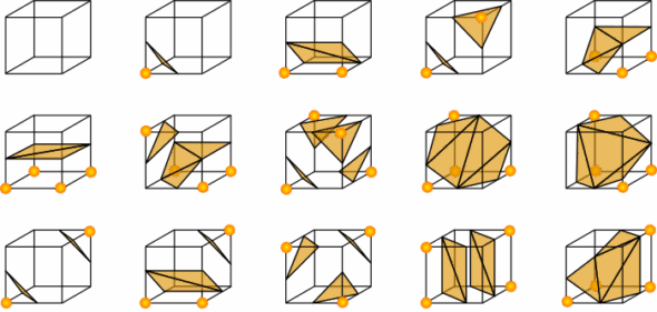
The 15 unique cube configurations
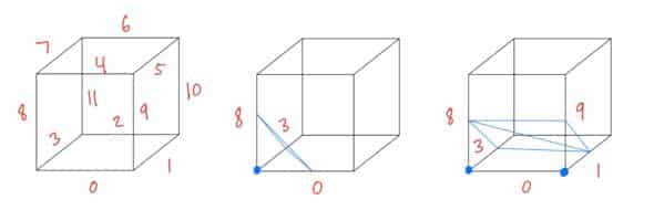
Each of the cube’s 12 edges is assigned a numeric label (see figure below). The values stored in the triangulation table refer to the edges by their label. One example of a triangulation entry is (00000001, [0, 8, 3]). The key 00000001 indicates that only 1 corner is inside the surface. The value for that configuration is a list telling us that edges 0, 8, and 3 should be connected to form a triangle. (See the second cube in the figure below.)
Another example of an entry is (00000011, [3, 8, 1, 1, 8, 9]), where edges 0, 8, and 1 form a triangle, and edges 1, 8, and 9 form another triangle (the third cube in the figure below). Each triangulation list will have a length divisible by 3 and will contain 5 triangles.
Adding Polish
Note that in the figures above, the vertex of each triangle is at the midpoint of the cube’s edge. While placing the vertices at the midpoint is a valid approach, this usually results in a less smooth final mesh. To fix this, you can use linear interpolation to determine the point at which the isosurface intersects with each edge using the iso-value, the two vertices defining an edge, and the vertices’ scalar values. This interpolation adjusts the position of the triangle’s vertices to make the positioning more accurate.
The newly calculated position of the vertex is stored in a list of vertices. In turn, that’s added to a global list of vertices. Every 3 vertices in the list form a triangle.
By repeating this process for every cube in the scalar field, the resulting vertices list can generate a 3D mesh composed of triangles. Note that the marching cubes algorithm doesn’t actually create the mesh. The algorithm only outputs the information for the triangles.
Generating a Sphere to Display
First, import the following Python packages:
import numpy as np
import plotly.graph_objects as go
from skimage import measure # this is scikit-image
Now, you can use numpy to create an open mesh grid:
grid_size = 64
x, y, z = np.ogrid[-1:1:grid_size*1j, -1:1:grid_size*1j, -1:1:grid_size*1j]
In these two lines of code, we are using numpy’s ogrid() function to create coordinate arrays for x, y, and z ranging from -1 to 1 with a step size of grid_zize*1j in each dimension where x will have shape (grid_size, 1, 1), y will have shape (1, grid_size, 1), and z will have shape (1, 1, grid_size).
Using the formula for a sphere, x^2 + y^2 + z^2 = r^2, you can convert the grid into a scalar field:
sphere = (x**2 + y**2 + z**2)
sphere is now a 3D array where each (x, y, z) point corresponds to a scalar value.
Applying Marching Cubes
The sphere generated from the previous section can be passed into scikit-image’s marching_cubes() function to extract its vertices and faces. The first argument is the data volume, and the second argument is the iso-value:
radius = 0.5
vertices, faces, _, _ = measure.marching_cubes(sphere, radius**2)
You can unpack the vertices and faces like so:
# Vertex coordinates
x_coords = vertices[:, 0]
y_coords = vertices[:, 1]
z_coords = vertices[:, 2]

# Triangle face vertex indices
v0 = faces[:, 0]
v1 = faces[:, 1]
v2 = faces[:, 2]
To understand this output, let’s look at an example of possible values (this specific example happens to be a tetrahedron):
x_coords = [0, 1, 2, 0]
y_coords = [0, 0, 1, 2]
z_coords = [0, 2, 0, 1]
v0 = [0, 0, 0, 1]
v1 = [1, 2, 3, 2]
v2 = [2, 3, 1, 3]
x_coords, y_coords, and z_coords give us x, y, and z value of each vertex. In this case, we have 4 vertices: (0, 0, 0), (1, 0, 2), (2, 1, 0), and (0, 2, 1). v0, v1, and v2 give us the indices of the vertices that form triangles. For example, the first entry (0, 1, 2) tells us that the vertex at index 0 (0, 0, 0), index 1 (1, 0, 2), and index 2 (2, 1, 0) from the coordinate lists form a triangle.
Displaying the Mesh
Next, the extracted vertices and faces from the marching cubes algorithm can then be passed into plotly’s Mesh3D() function to create an object that can be displayed:
plotly_mesh = go.Mesh3d(
   x=x_coords,
   y=y_coords,
   z=z_coords,
   i=v0,
   j=v1,
   k=v2,
   color="red"
   )
Finally, the mesh can be displayed in the browser:
fig = go.Figure(data=plotly_mesh)
fig.update_layout(title="Marching Cubes Example")
fig.show()

The resulting mesh is very smooth-looking thanks to the interpolation. Printing the length of faces reveals that this sphere is made up of 9,452 triangles. In other words, the more triangles there are, the smoother the mesh will look.
As an optional step, this figure can also be saved as an HTML file to view later without needing to rerun the script:
fig.write_html("example.html")
View the code used for this tutorial in the following GitHub repo:
github.com/georgia-martinez/atomic-spin-projects/tree/main/project2_marching_cubes